
Rolling Statistics
Peforms rolling statistics analysis on assets. Analysis on Portfolios not supported yet.
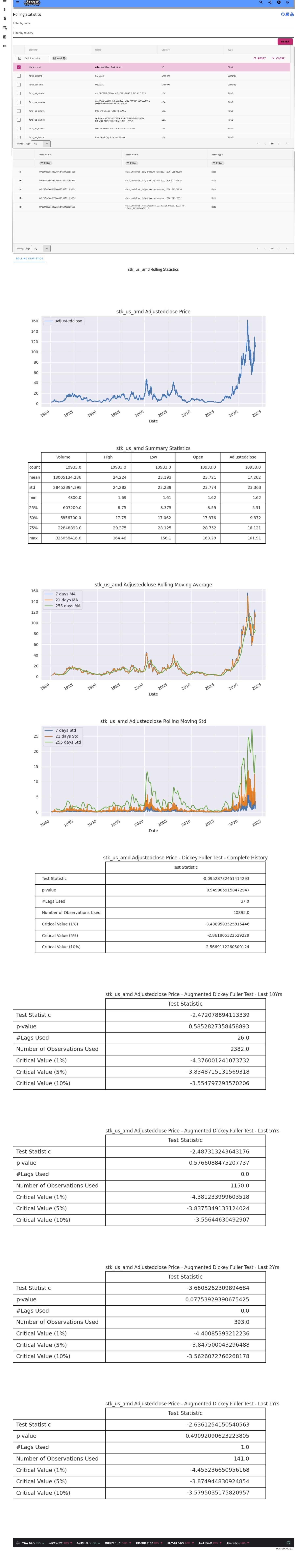
Rolling Statistics - Screenshot
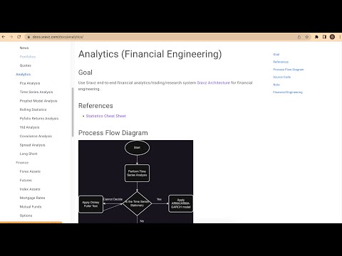
Code explanation video
Source Code
Use case
Perform Dicky Fuller Test to check if a timeseries is stationary or non stationary
Stationary Process: A process that generates a stationary series of observations.
Stationary Model: A model that describes a stationary series of observations.
Trend Stationary: A time series that does not exhibit a trend.
Seasonal Stationary: A time series that does not exhibit seasonality.
Strictly Stationary: A mathematical definition of a stationary process, specifically that the joint distribution of observations is invariant to time shift.
- Last Price Chart displays asset last price
- Summary statistics displays statistics on the asset timeseries.
- Count: Show number of data points in the timeseries
- Mean: Mean last price
- Std: Std last price
- Min: Min last price
- 25%: First quartile of the last price distribution
- 50%: Second quartile of the last price distribution
- 75%: Thrid quartile of the last price distribution
- Max: Max last price
- Displays moving average plots.
- 7 days MA: 7 days Moving Average Plot
- 21 days MA: 21 days Moving Average Plot
- 255 days MA: 255 days Moving Average Plot
- Displays moving std plots.
- 7 days std: 7 days Moving Standard Deviation Plot
- 21 days std: 21 days Moving Standard Deviation Plot
- 255 days std: 255 days Moving Standard Deviation Plot
- Augmented Dickey-Fuller unit root test.
- Auto Regressive Model with no time trend
$$ y_{t}=\rho y_{t-1}+u_{t}\, $$
$$ \Delta y_{t}=(\rho -1)y_{t-1}+u_{t}=\delta y_{t-1}+u_{t} $$
Unit Root is present if:$$ \delta = 0 $$
- The null hypothesis of the test is that the time series can be represented by a unit root, that it is not stationary (has some time-dependent structure).
- A stationary timeseries will have a constant mean, standard deviation and no sesonality
- The alternate hypothesis (rejecting the null hypothesis) is that the time series is stationary.
- p-value is the smallest level of significance at which the null hypothesis would be rejected
- p-value > 0.05: Fail to reject the null hypothesis (H0), the data has a unit root and is non-stationary.
- p-value <= 0.05: Reject the null hypothesis (H0), the data does not have a unit root and is stationary.
- Auto Regressive Model with time trend
$$ \Delta y_t = \alpha + \beta t + \gamma y_{t-1} + \delta_1 \Delta y_{t-1} + \cdots + \delta_{p-1} \Delta y_{t-p+1} + \varepsilon_t, $$
where $$\alpha$$ is a constant,$$ \beta $$
the coefficient on a time trend and$$ p $$
the lag order of the autoregressive process. Imposing the constraints$$ \alpha = 0\ \&\ \beta = 0 $$
corresponds to modelling a random walk and using the constraint$$ \beta = 0 $$
corresponds to modeling a random walk with a drift.
- Auto Regressive Model with no time trend