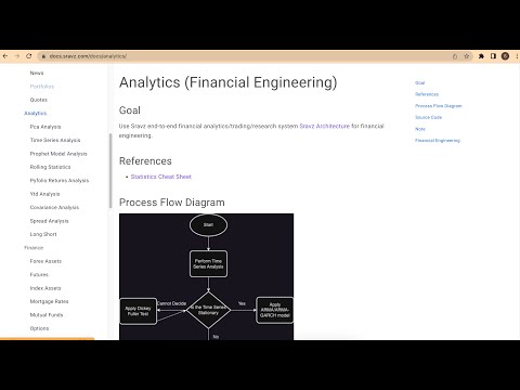
Principal Component Analysis (PCA)

Performs PCA on portfolios and visualizes the PCA report.

PCA Analysis

Sravz PCA Analysis - Screenshot

Screenshot:

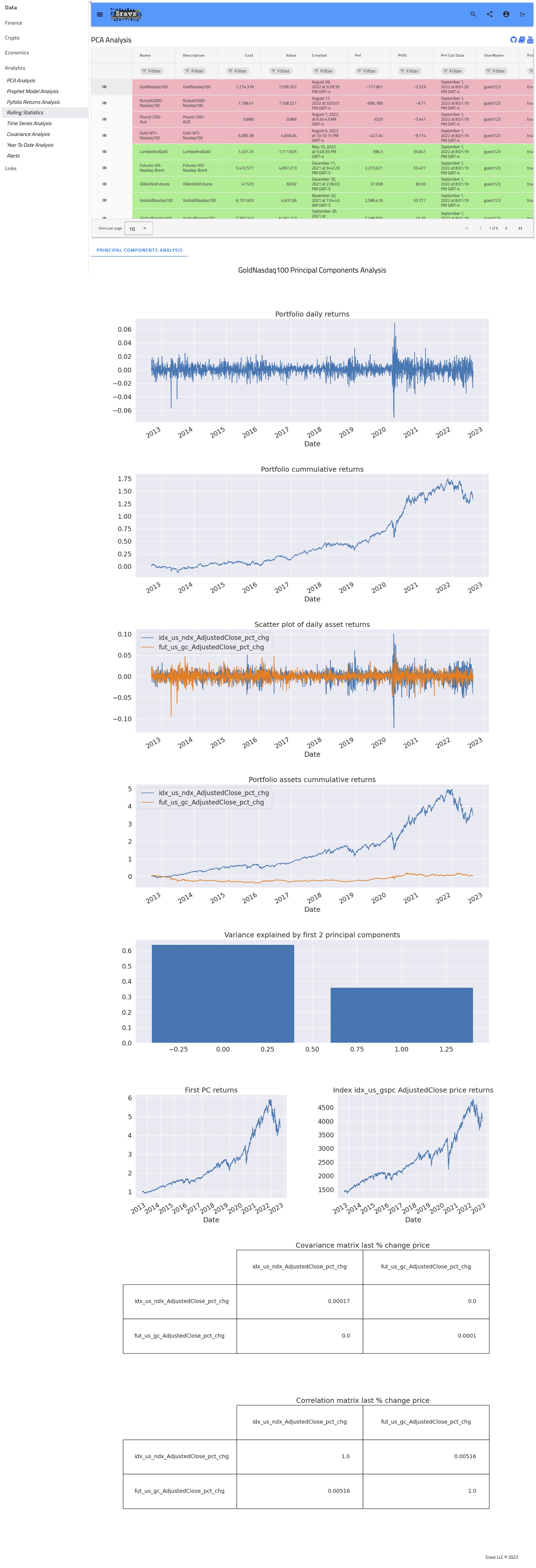
What the PCA Analysis Page Shows

Portfolio selector (for assetType=portfolio).
PCA Report tab with an interactive Plotly report for the selected portfolio.
Covariance/Correlation analysis (when available) rendered as a matrix table.

Backend Behavior

Uses PCA_ENGINE.create_portfolio_pca_report to generate the PCA report.
The backend returns a Plotly JSON report, which the frontend renders directly in the UI.
For public portfolios without a user ID, the report is generated using the portfolio asset list passed from the UI.

Use Cases (Finance)

Identify Dominant Risk Factors

PCA decomposes the portfolio return covariance matrix into orthogonal components that represent independent sources of risk. In a multi-asset portfolio the first few principal components typically map to well-known macro risk factors — interest rate duration, broad equity beta, credit spreads, and commodity cycles. By inspecting the eigenvector loadings you can label each PC and quantify what fraction of total portfolio variance each macro factor explains, replacing hundreds of correlated positions with a compact factor view.

Three plots in the PCA report directly support this:

Explained Variance Bar Chart (Variance explained by first N principal components) — each bar is one PC. A bar that towers above the rest immediately identifies the dominant risk factor. If PC1 captures 60 % of variance, a single macro theme (usually broad equity beta) drives most of your portfolio’s risk. The cumulative sum of bars tells you how many independent factors you need to model before you account for, say, 90 % of total variance.

First PC Returns vs Benchmark Index (First PC returns / Index price returns) — the left subplot is the cumulative return of a synthetic portfolio weighted by the PC1 eigenvector loadings; the right subplot is the benchmark index price. High co-movement between the two confirms that PC1 represents the market/equity-beta factor. Divergence between them signals that a different macro theme (rates, commodities, credit) is the true first factor for your specific portfolio.

Correlation Matrix (Covariance matrix last % change price) — assets that share the same dominant PC will show high pairwise correlation in this table. Blocks of high correlation identify clusters of assets that are all expressing the same risk factor, making it easy to label each PC by looking at which asset cluster loads heavily on it.

Detect Redundant Holdings

When two or more assets load heavily on the same principal component with similar signs, they are essentially expressing the same risk. PCA surfaces these overlaps even when the assets appear superficially different (e.g., a tech ETF and a growth-factor fund). Removing or trimming the redundant leg reduces trading costs and concentration risk without materially changing the portfolio’s risk profile.

Dimensionality Reduction for Factor-Based and Risk-Parity Allocations

A portfolio of N assets has an N×N covariance matrix that is noisy and hard to invert stably. Projecting onto the top K principal components (where K « N) filters estimation noise and yields a cleaner risk model. This lower-dimensional representation feeds directly into:

Factor-based allocation — weight assets by their PC scores to tilt toward desired risk themes.
Risk-parity — equalise risk contribution across the retained PCs rather than across individual assets, producing more balanced diversification.

Stress Test Sensitivity During Regime Shifts

Each principal component can be shocked independently. Applying a +2σ or +3σ shock to PC1 (e.g., a rate spike) and observing P&L impact across the portfolio replicates the kind of macro stress that was historically hardest to hedge. Because PCs are orthogonal, you can isolate the pure effect of each factor without contamination from the others — something that is impossible with correlated raw-asset shocks.

Compare Diversification Across Portfolio Construction Methods

The cumulative explained-variance curve (scree plot) is a single, comparable metric for diversification quality. A portfolio where PC1 explains 80 % of variance is far less diversified than one where the first five PCs are roughly equal. Running PCA on multiple candidate portfolios (equal-weight, mean-variance, minimum-variance, risk-parity) and overlaying their scree plots gives an immediate, model-free ranking of their true diversification.

Build Hedges by Neutralizing Principal Component Exposures

To hedge out a specific macro risk, compute the portfolio’s loading on the corresponding PC and construct an offsetting position whose loading is equal and opposite. For example, if PC1 represents duration risk and the portfolio has a large positive loading, a short position in interest-rate futures sized by the eigenvector weight neutralizes that exposure while leaving equity and credit bets intact. This systematic approach replaces ad-hoc hedging with a mathematically grounded framework tied directly to observed return co-movements.

PCA Basics

Dimensionality reduction technique.
PCA is performed on symmetric correlation or covariance matrices. $$$ Corr(X,Y)=Corr(Y,X) $$$ $$$ Cov(X,Y)=Cov(Y,X) $$$
Covariance matrix is a square matrix giving the covariance between each pair of assets in a portfolio daily returns vector. Main diagonal contains variances (covariance with itself).
Correlation matrix is a square matrix giving the correlation between each pair of assets in a portfolio daily returns vector. Main diagonal contains correlations (each asset with itself = 1).
Correlation and covariance are positive when variables move together and negative when they move in opposite directions.
The covariance matrix defines the spread (variance) and the orientation (covariance) of the dataset. The direction of the spread is computed by eigenvectors and its magnitude by eigenvalues.
k-dimensional data has k principal components (each asset’s daily returns contributes to a component).
Principal components are linear uncorrelated variables (orthogonal matrix): $A^{\top}A = AA^{\top} = I$
If T is a linear transformation from a vector space V over a field F into itself and v is a nonzero vector in V, then v is an eigenvector of T if T(v) is a scalar multiple of v. This can be written as: $T(v)=\lambda(v)$ where λ is a scalar in F, known as the eigenvalue, characteristic value, or characteristic root associated with v.
Perform linear transformation on the covariance matrix $\begin{bmatrix} Var(x) & Cov(x,y)\\ Cov(y,x) & Var(y) \end{bmatrix}\begin{bmatrix} v_1\\ v_2 \end{bmatrix}^T=\begin{bmatrix} \lambda_1\\ \lambda_2 \end{bmatrix}\begin{bmatrix} v_1\\ v_2 \end{bmatrix}$ where $$$ v_1,v_2... $$$ are eigenvectors and $\lambda_1,\lambda_2...$ are eigenvalues

Code explanation video

Source Code

Principal Component Analysis